Part 1 – Getting familiar with hyperspectral imaging data analysis – loading the data.

A friend of mine was recently hired as a graduate software developer in a company that specializes in hyperspectral imaging (HSI). This is when I first heard about this technology.

While I did not give much thought initially (I didn’t really know what it was), the more he spoke about it the more interested I became. From our conversations I was beginning to learn about its primary functions and how widely applicable the HSI is. It blew my mind.

Hyperspectral imaging is technique of collecting and processing large number of images of the same spatial area at different wavelengths. HSI obtains the spectrum for each pixel in the image of an area.

The collected data forms what is called a hyperspectral cube, where two dimensions represent the area while third dimension represents the spectral content.

I went on a quest of looking for more information about the subject in a more programming related context. I have found that the availability of sample data is somehow limited. There was also not many programming related training materials and the ones that I have found did not provide much context about the methods used.

Let’s get started.

I managed to find a dataset of hyperspectral images that were made available by Pavia University from Italy. The dataset consist of 103 spectral bands and the size of the image is 610×340 pixels. Data also contained the the ground truth with 9 classes.

The data was provided in format of ‘mat’ files that needed to be loaded first. After a quick check I found that I can use the Python SciPy for that.

from scipy.io import loadmat 
import matplotlib.pyplot as plt

# load sample data
img_data = loadmat('data/PaviaU.mat')

After loading the sample data I wanted to actually visualize it as well as to check its structure.

def display_band():
    # check for keys
    data_keys = list(img_data.keys())
    print(data_keys)

Getting the data from index 3 and examining the shape.

# get data from index 3 - the 'paviaU'
data_In = (img_data[data_keys[3]])
print(data_In.shape)

This has confirmed that for each of 103 bands images are 610×340 pixels (this represents the two dimensional area) and the 103 represents the spectral content.

To visualize sample band image I used the matplotlib pyplot library.

# set size for convenience
plt.figure(figsize(8,8))
# image/band at index 0
plt.imshow(data_In[:,:,0])
plt.show()

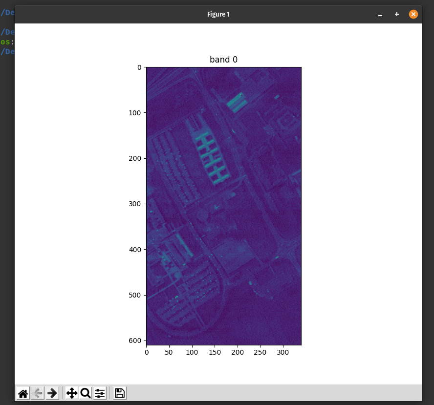
We can also take a look at few other bands.

This allowed me to take a quick look at the data: load, check for keys, examine the shape and visualise some of the samples.

from scipy.io import loadmat 
import matplotlib.pyplot as plt


# load the data
img_data = loadmat('data/PaviaU.mat')

# examine and visualize
def display_band():
    # check data
    #print(img_data)
    
    # check for keys
    data_keys = list(img_data.keys())

    # data from index 3: 'paviaU'
    data_In = (img_data[data_keys[3]])

    # check shape
    print(data_In.shape)

    # visualise sample image/band at index 0
    plt.figure(figsize=(8,8))
    plt.imshow(data_In[:, :, 0])
    plt.show()

Part 2: Getting started with exploration and analysis.