
Loading the data and check shape.
The Pavia University provided dataset includes the samples as well as the ground truth.
def load_data():
    '''
    X - input: 3D
    y - output: 2D
    '''
    X = loadmat('data/PaviaU.mat')['paviaU']
    y = loadmat('data/PaviaU_gt.mat')['paviaU_gt']
    print("X shape: ", X.shape)
    print("y shape: ", y.shape)
    return X, y

X, y = load_data()

To analyse HSI data I needed to remember that this image data has some differences from the regular cat, dog, human classification problem. HSI is high-dimensional and it took me a short while to wrap my head around this….
The valuable data in HSI is in the spectral content of the pixel which can be used as a unique “fingerprint” to identify materials and/or quality.
To understand it better and to expand on the initial visualisation of the spectral bands in part 1 it could also be explained as: each pixel is a vector of the length of the number of bands of HSI.
To extract this data from pixels we need to reshape it/turn it into a vector.
This can be done automatically by using the reshape() method by providing it with the parameters:
‘-1’ (unknown: which lets the method to figure it out)
and
‘X.shape[2]’ (the shape at index 2: which is 103 in this case)
def get_pixels(X, y):
    # extract pixels/reshape:
    # each pixel is a vector of length of the number of bands of HSI

    # examine the data and shape of X sample
    print("X0")
    print(X[0])
    print("X0 shape")
    print(X[0].shape, "\n")


    # reshape
    q = X.reshape(-1, X.shape[2])

    # examine the data and shape after reshape
    print("Q0")
    print(q[0])
    print("Q0 shape")
    print(q[0].shape, "\n")

    # X shape
    print("X-shape ", X.shape)
    # q shape
    print("q-shape ", q.shape)


    # '''
    # q shape:  (207400, 103)
    # 610x340
    # '''
As we can see the reshape() method allowed to turn it into a vector.

This is the part where I still need to do some more research to gain a deeper understating of the spectral dimension as it’s still a little unclear to me but since I now have a vector I could not just leave it without plotting it on a graph 🙂 .
We can use matplotlib pyplot to do this.
    # plot the q[0] vector
    plt.plot(q[0])
    plt.show()

    # plot the q[80] vector
    plt.plot(q[80])
    plt.show()

Making the data frame using Pandas library.
Now that I have the vectors it’s time to make a data frame and make space for the classes.
# data frame
# loading our 'q' as 'data'
df = pd.DataFrame(data = q)
# dataframe with classes
# concatenate data and space for classes
df = pd.concat([df, pd.DataFrame(data = y.ravel())], axis = 1)
# column names
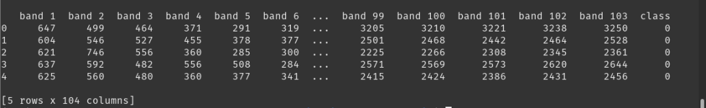
df.columns = [f'band {i}' for i in range(1, X.shape[2] + 1)] + ['class']
# display the data-frame head (5 rows)
print(df.head())
# save to csv file
df.to_csv('data_set.csv')
return df
The code:
# gettin the pixels and saving to csv file
def get_pixels(X, y):
    # extract pixels/reshape:
    # each pixel is a vector of length of the number of bands of HSI
    print('X0 shape')
    print(X[0].shape, '\n')

    q = X.reshape(-1, X.shape[2])
    print('Q0 shape')
    print(q[0].shape, '\n')

    # X shape
    print('X-shape ', X.shape)
    # q shape
    print('q-shape ', q.shape, '\n')

    # plot vector at index q[0]
    plt.plot(q[0])
    plt.show()

    '''
    print('q shape: ', q.shape)
    q shape:  (207400, 103)
    610x340
    '''

    # data frame
    df = pd.DataFrame(data = q)

    # dataframe with class column
    df = pd.concat([df, pd.DataFrame(data = y.ravel())], axis = 1)

    # column names
    df.columns = [f'band {i}' for i in range(1, X.shape[2] + 1)] + ['class']

    # store to csv file
    df.to_csv('data_set.csv')
    return df


df = get_pixels(X, y)
print(df.head())
In the next Part 3 of my exploration of HSI I will do some more data exploration and visualization. Also, since HSI data is high dimensional, I will touch on some more complex subjects such as dimension reduction using PCA (I’m still doing some research on that to understand it more). Stay tuned.
