Part 3 – Analysing Data, Preparation, Dimension Reduction and Visual Exploration

In the last part a data frame was created.

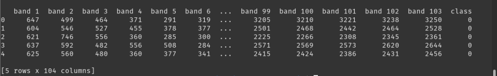
This data has many dimensions and if we wanted to plot it in its current form it could prove difficult.

I have not previously worked with this kind of data so I had to look things up. Fortunately I have found a blog post about working with hyperspectral data here. It had a great deal of information and code for someone that begins to learn about HSI but most of the content did not explain how the used methods work or why use them. I did some additional research on those and I will include the list of interesting sources at the end of this post….

Reducing the dimensions with Principal Component Analysis or PCA.

This is something I need to investigate further to gain deeper understanding of but PCA is often used in statistics and in working with high dimensional data as a way to reduce the dimensionality of feature space. The Royal Society Publishing website defines PCA as:

Large datasets are increasingly common and are often difficult to interpret. Principal component analysis (PCA) is a technique for reducing the dimensionality of such datasets, increasing interpretability but at the same time minimizing information loss.
https://royalsocietypublishing.org/doi/10.1098/rsta.2015.0202

Also, here are few sources with more in depth information abut this method:

1. StatQuest: Principal Component Analysis (PCA), Step-by-Step

https://www.youtube.com/watch?v=HMOI_lkzW08

2. StatQuest: PCA main ideas in only 5 minutes!!!

https://www.youtube.com/watch?v=FgakZw6K1QQ

and

3. Visualising the Classification Power of Data using PCA

https://towardsdatascience.com/visualising-the-classification-power-of-data-54f5273f640

Lets get back to the data.

The dimension reduction with PCA was already implemented in the sklearn library which means it can just be imported and used.

from sklearn.decomposition import PCA

# PCA
pca = PCA(n_components=3)

# apply PCA and update data frame
# data.iloc[<row selection>, <column selection>] //remove
dt = pca.fit_transform(df.iloc[:, :-1].values)

To check the result we can print out a sample row, let’s print the last one at index 207399:

print('dt 207399 ', dt[207399])

This results in three principal components.

Next step is to concatenate the data add space for class.

# concatenate the data and the classes
q = pd.concat([pd.DataFrame(data = dt), pd.DataFrame(data = y.ravel())], axis = 1)

# set column names
q.columns = [f'PC - {i}' for i in range(1, 4)] + ['class']

print(q.head())

We now have 3 dimensions.

Saving data to csv file.

# save to csv file
q.to_csv('data_set_pca.csv', index=False)

We can remove class 0, take a look at value counts and then create labels:

# remove class 0
qq = q[q['class'] != 0]

# check counts for classes
print(qq['class'].value_counts())

# labels
labels = {'1': 'Asphalt',
'2' :'Meadows',
'3'	:'Gravel',
'4'	:'Trees',
'5'	:'Painted metal sheets',
'6'	:'Bare Soil',
'7'	:'Bitumen',
'8'	:'Self Blocking Bricks',
'9'	:'Shadows'}

We can now assign the labels, check the counts again and see the result.

# add class labels column
qq['labels'] = qq['class'].apply(lambda x: labels[str(x)])

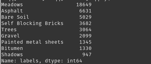
# check counts for classes
print(qq['labels'].value_counts())

# chck head
print(qq.head())

Value counts:

With labels:

And resulting data-frame head:

Visualise class distribution

# set the bar plot with class labels
plt.bar(range(len(counts)), counts, tick_label=counts.index)
# set the title
plt.title('Class Distribution')
# show the plot
plt.show()